Simple Linear Regression with R
- Using Women's Height to predict Women's Weight
(Bee's revision summary note, completed 13 March 2017)
This analysis is done using R and knitr package(for the html compilation).
Main textbook reference for this summary:
"R In Action, Data analysis and graphics with R." - by Rober I. Kabacoff (ISBN: 9781617291388)
My summary here is done following the above mentioned book, with some additional study notes and codes added for my own reference.
For more comprehensive explanation, do refer to the book instead. The book is available on Amazon.
The goal of the analysis in this summary is to determine whether we can predict weight from height, based on the dataset "women" provided in base R installation, using Simple Linear Regression method.
Simple Linear Regression is a linear regression model with a single explanatory variable; using one quantitative explanatory variable to predict a quantitative outcome, or response variable. It is the simpliest form of Regression model.
1) Input Dataset
The dataset "women" gives the average heights and weight for American women aged 30-39.
The dataset consists of a dataframe with 15 observations on 2 variables:
- height numeric Height (in)
- weight numeric Weight (lbs)
Data Source: The World Almanac and Book of Facts, 1975.
Structure of the data:
str(women)
## 'data.frame':	15 obs. of  2 variables:
##  $ height: num  58 59 60 61 62 63 64 65 66 67 ...
##  $ weight: num  115 117 120 123 126 129 132 135 139 142 ...
As I am more familiar with cm and kg, will convert the dataset from inch to cm and from lbs to kg:
- 1 inch = 2.54 cm
- 1 lbs (pound) = 0.453592 kg
Structure of the data:
women$height <- women$height*2.54
women$weight <- women$weight*0.453592
str(women)
## 'data.frame':	15 obs. of  2 variables:
##  $ height: num  147 150 152 155 157 ...
##  $ weight: num  52.2 53.1 54.4 55.8 57.2 ...
Summary Statistics of the data:
summary(women)
##      height          weight
##  Min.   :147.3   Min.   :52.16
##  1st Qu.:156.2   1st Qu.:56.47
##  Median :165.1   Median :61.23
##  Mean   :165.1   Mean   :62.02
##  3rd Qu.:174.0   3rd Qu.:67.13
##  Max.   :182.9   Max.   :74.39
2) Plots
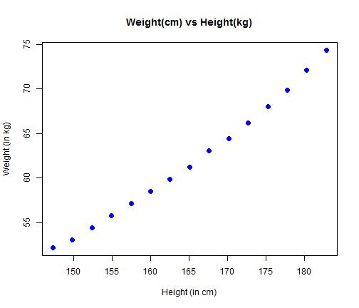
The basic scatter plot for the dataset (weigth vs height), using Base R plot function.
plot(women,
     main="Weight(cm) vs Height(kg)",
        xlab="Height (in cm)",
        ylab="Weight (in kg)",
     pch=16,cex=1.3,col="blue")
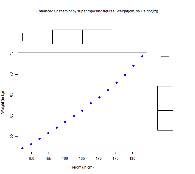
We can also enhance the plot by superimposing several figures into a single plot, to help us understand the distribution better.
par(fig=c(0,0.8,0, 0.8))
plot(women$height,women$weight,
        pch=16,cex=1.3,col="blue",
        xlab="Height (in cm)",
        ylab="Weight (in kg)")
par(fig=c(0,0.8,0.55,1), new=TRUE)
boxplot(women$height, horizontal=TRUE,axes=FALSE)
par(fig=c(0.65,1,0,0.8), new=TRUE)
boxplot(women$weight, axes=FALSE)
mtext("Enhanced Scatterplot by superimposing figures, Weight(cm) vs Height(kg)",side=3,outer=TRUE,line=-3)
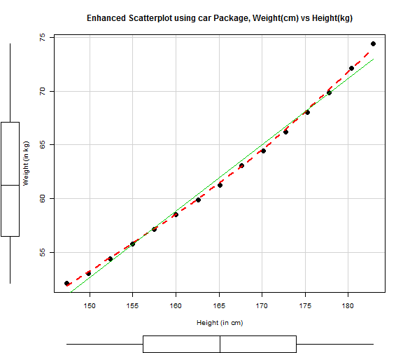
The simpler approach to create an enhance scatter-plot will be to use the scatterplot() function in the car package.
library(car)
## Warning: package 'car' was built under R version 3.2.5
scatterplot(weight~height,data=women,
            spread=FALSE, smoother.args=list(lty=2),
            pch=19,cex=1.6,
            xlab="Height (in cm)",
            ylab="Weight (in kg)",
            main="Enhanced Scatterplot using car Package, Weight(cm) vs Height(kg)"
            )
3) Simple Linear Regression
The function lm() is used to fit lnear models and carry out regression analysis.
fit <- lm(weight~height,data=women)
Result of lm as follows:
summary(fit)
##
## Call:
## lm(formula = weight ~ height, data = women)
##
## Residuals:
##     Min      1Q  Median      3Q     Max
## -0.7862 -0.5141 -0.1739  0.3364  1.4137
##
## Coefficients:
##              Estimate Std. Error t value Pr(>|t|)
## (Intercept) -39.69686    2.69295  -14.74 1.71e-09 ***
## height        0.61610    0.01628   37.85 1.09e-14 ***
## ---
## Signif. codes:  0 '***' 0.001 '**' 0.01 '*' 0.05 '.' 0.1 ' ' 1
##
## Residual standard error: 0.6917 on 13 degrees of freedom
## Multiple R-squared:  0.991,	Adjusted R-squared:  0.9903
## F-statistic:  1433 on 1 and 13 DF,  p-value: 1.091e-14
Use fitted() to extract the model fitted values:
fitted(fit)
##        1        2        3        4        5        6        7        8
## 51.06690 52.63179 54.19668 55.76158 57.32647 58.89136 60.45625 62.02115
##        9       10       11       12       13       14       15
## 63.58604 65.15093 66.71582 68.28072 69.84561 71.41050 72.97539
Use residuals() to extract the model residual values:
residuals(fit)
##            1            2            3            4            5
##  1.096180667  0.438472267  0.234355867  0.030239467 -0.173876933
##            6            7            8            9           10
## -0.377993333 -0.582109733 -0.786226133 -0.536750533 -0.740866933
##           11           12           13           14           15
## -0.491391333 -0.241915733  0.007559867  0.710627467  1.413695067
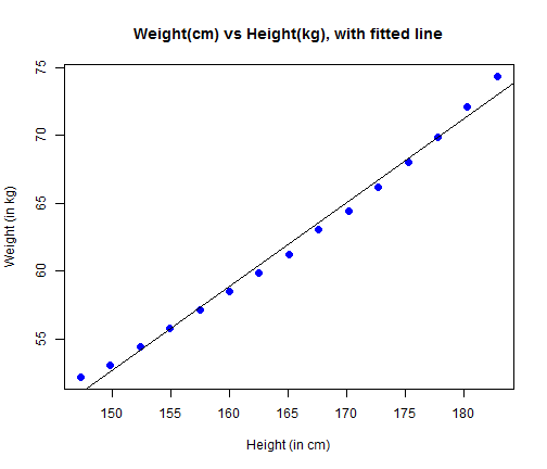
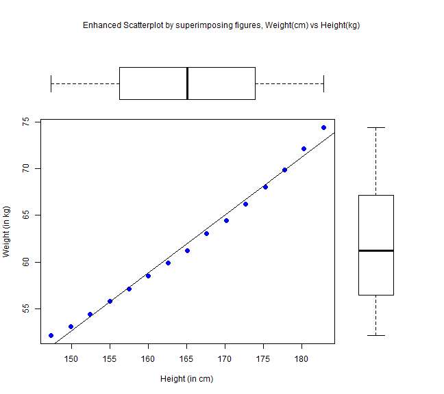
Plot the scatter plot with a fitted line using abline() (function to add straiht lines to plot).
plot(women$height, women$weight,
     main="Weight(cm) vs Height(kg), with fitted line",
     pch=16,cex=1.3,col="blue",
        xlab="Height (in cm)",
        ylab="Weight (in kg)")
abline(fit)
par(fig=c(0,0.8,0, 0.8))
plot(women$height,women$weight,
        pch=16,cex=1.3,col="blue",
        xlab="Height (in cm)",
        ylab="Weight (in kg)")
abline(fit)
par(fig=c(0,0.8,0.55,1), new=TRUE)
boxplot(women$height, horizontal=TRUE,axes=FALSE)
par(fig=c(0.65,1,0,0.8), new=TRUE)
boxplot(women$weight, axes=FALSE)
mtext("Enhanced Scatterplot by superimposing figures, Weight(cm) vs Height(kg)",side=3,outer=TRUE,line=-3)
4) Conclusion
summary(fit)
##
## Call:
## lm(formula = weight ~ height, data = women)
##
## Residuals:
##     Min      1Q  Median      3Q     Max
## -0.7862 -0.5141 -0.1739  0.3364  1.4137
##
## Coefficients:
##              Estimate Std. Error t value Pr(>|t|)
## (Intercept) -39.69686    2.69295  -14.74 1.71e-09 ***
## height        0.61610    0.01628   37.85 1.09e-14 ***
## ---
## Signif. codes:  0 '***' 0.001 '**' 0.01 '*' 0.05 '.' 0.1 ' ' 1
##
## Residual standard error: 0.6917 on 13 degrees of freedom
## Multiple R-squared:  0.991,	Adjusted R-squared:  0.9903
## F-statistic:  1433 on 1 and 13 DF,  p-value: 1.091e-14
- Based on the output, the model is: weight = -39.69686 + (0.61610*height)
- R2=0.991 indicates that the model accounts for 99.1% of the variance in weights.
- F-Statistic, p-value: 1.091e-14
The hypotheses:
Null hypothesis: The fit of the intercept-only model and the fitted model are equal.
Alternative hypothesis: The fit of the intercept-only model is significantly reduced compared to the model.
Since the P value for the F Statistics is less 0.05, i.e. the significance level set at 95% confidence, we reject the null-hypothesis and conclude that the model is a better fit than the intercept-only model (or random model, i.e. the mean of the response).
- T-Statistics for height, p-value: 1.09e-14 ***
The F-test is equivalent to the T-test for height in this case because there is only one explanatory variable.
To conclude, based on the F-Statistic, the model is acceptable. However, if we look at the model plot, it seems that the linear model may not be the best model; the shape of the plot suggest that a polynomial model with quadratic term may give a better fit.
@The end.